Dynamic Programming

Abstract

---

• Also known as Dynamic Optimisation
• Divide a given problems into smaller problems, answers to those smaller problems generate the answer to the given problem. We make use of Memoization to remember the answers to those smaller problems, so we don’t re-solve those smaller problems

Dynamic

I wanted to get across the idea that this was dynamic, this was multistage, this was time-varying. - Bellman

So Dynamic programming is also known as Multistage Optimisation. The multstage here refers to the stages of solving subproblems which deliver the final optimal answer to a given problem.

• There are two main approaches to DP algorithms - Top-down DP Approach and Bottom-up Approach

DP Debugging

Print out DP Table to check any errors.

Question Bank

Basics

• 509. Fibonacci Number

Statelessness (无后效性)

• 455A - Boredom (1500)

Continuous Sub-sequence

• 628B - New Skateboard (Number Theory Required)

Simulation

• 1766C - Hamiltonian Wall

Top-down DP Approach

---

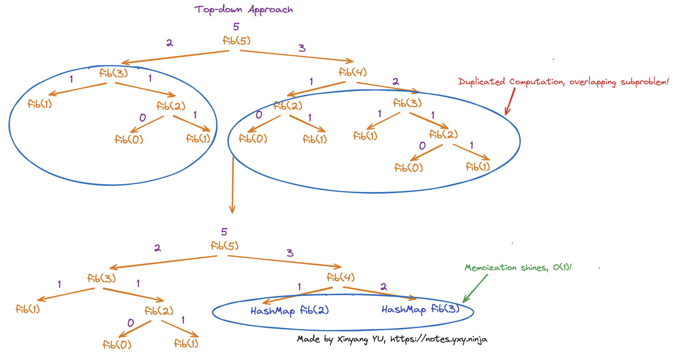
• Start with the large, complex problem, and understand how to break it down into smaller subproblems, perform Memoization by recording down the answer of subproblems to avoid duplicated computation on overlapping subproblems. Above shows how can we make use of top-down approach to find Fibonacci sequence in $O(n)$

Attention

The space complexity of Top-down approach is $O(n)$, we need to record down the answer for all the subproblems.

When we break down the larger problem into smaller subproblems, some subproblems may already be solved but some aren’t. The size of subproblems can vary, so we have to record down the answer to each solved subproblems, so we can solve that subproblem in$0(1)$ if we see that subproblem again.

Divide and Conquer

• Top-down DP Approach without Memoization, because overlapping subproblems aren’t a requirement for the Divide and Conquer approach
• Make use of Recursion to divide a given problem into smaller subproblems until its smallest form whose answer is known. We combine the answers of smaller subproblems into the answer of a bigger subproblem when the function calls on the smaller subproblems return

Example

Merge Sort

Bottom-up DP Approach

---

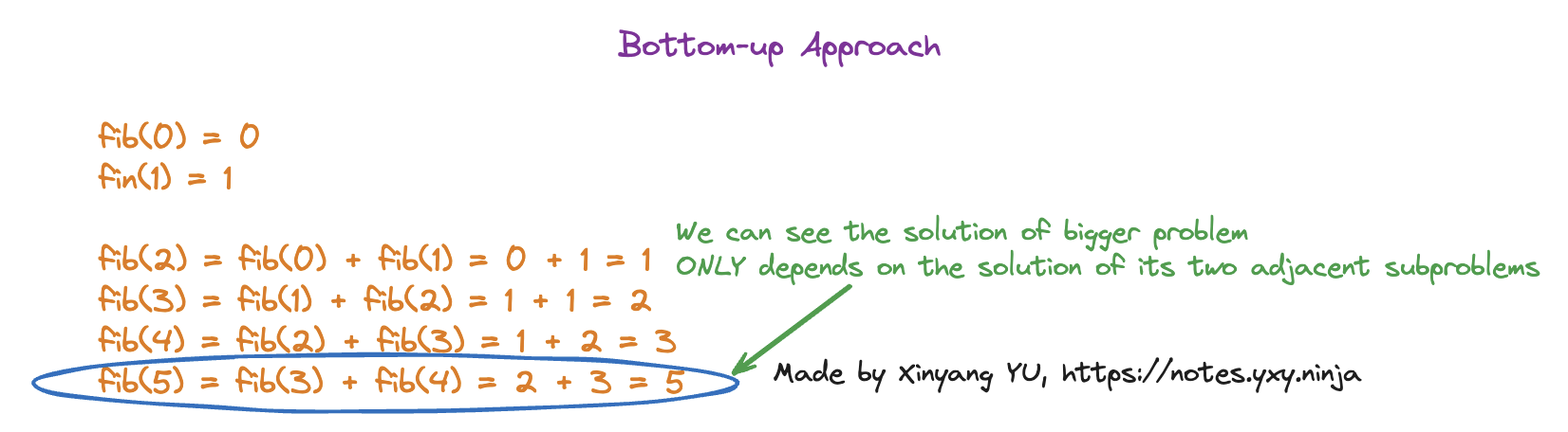
• Start with the smallest possible subproblems, figures out the solution to them, and then slowly builds itself up to solve the larger, more complicated subproblem

Space efficient

The space complexity of Bottom-up approach is $O(1)$, we just need to save the solutions of adjacent subproblems to obtain the answer to the bigger problem.

It is like finding the solution to $(5+5+5+5)+5$, we already know $(5+5+5+5)$ is $20$, then the answer to $(5+5+5+5)+5$ is simply $(20)+5$ which is $25$. You see we don’t need to remember what is the answer to $5+5$ or $5+5+5$, because the answer of $(5+5+5+5)+5$ depends directly on $(5+5+5+5)$, nothing else.

DP Problem Properties

---

Overlapping Subproblems (重复子问题)

• Occur when a problem can be broken down into smaller subproblems that are exactly the same

Tip

Overlapping subproblems can be handled efficiently with Memoization.

Optimal Substructure (最优子结构)

• When a problem has optimal substructure, we can use the optimal solutions of the subproblems to construct the optional solution of the given problem

Knapsack Problem

The solution can be found by building on the optimal solutions to the knapsack problem with smaller weights and values.

Statelessness (无后效性)

• Solutions to smaller problems are deterministic. 给定一个确定的状态， 其未来发展只与该状态有关， 与该状态所经历的过去的所有状态无关. 如果未来发展与该状态和该状态的前一个状态相关，我们可以靠矩阵来解。但如果回溯的状态过多，就难了
• 许多Backtracking problems 都不具有无后效性， 无法使用 Dynamic Programming 快速求解

State Transition Equation (状态转移方程)

---

• The mathematical operation we need to perform to transit from one state (smaller subproblems) to the next state (bigger subproblems), obtain the optimal solution of the problem eventually

0-1 knapsack problem

In 0-1 knapsack problem, the scope is basically the number of the items we can select. The less the items available to be selected the smaller the scope.

The smallest scope is $0$ item, in this case, the maximum value we can obtain is always $0$ regardless the size of the knapsack bag.

Then we expand the scope from $0$ item to $1$ item. What is the mathematical operation we need to perform to obtain the new state of the new scope?

The answer is to loop through the knapsack size from $1$ to the maximum size. At each size, if the weight of the new item exceeds the knapsack size, we get a bigger knapsack size until we get one that is big enough for the new item. The new state in this case is just the state of the previous smaller scope.

When the knapsack size is big enough, there are 2 choices for us, it is either we put the new item into the bag or we don’t. So how? Remember we want to maximise the value we can have inside the knapsack bag, so we should always make the decision that increments the value in the new state.

Lets abstract the problem:

• Let $s$ be the current knapsack bag size
• Let $p$ be the previous state with $s$, basically the best value we can have with $s$
• Let $w$ be the weight of the new item
• Let $v$ be the value of new item

So now we want to perform state transition which is to obtain the best value with bigger scope at $s$. How should we do that?

The answer is simple, we only put the new item into the knapsack bag if it can generate a bigger value at $s$.

We know the previous state is the best state at that smaller scope. So we can build on top of it! If I put in the new item, the best value it can generate is basically the best value at $s-w$ at the previous state(let this best value be $q$) + $v$. If we don’t put the new item, the best value is basically $p$.

Thus, we obtain our State Transition Equation. The new state at $p$ is Math.max(q + v, p). We put the new item into the bag if $q+v>p$, else we don’t.